Ultralytics YOLO: Giving Python a Pair of Eyes — Part I

Computer vision used to have a steep entry fee. Before we could detect one dog in one photo, we had to learn a pile of theory, assemble a model, find weights, write preprocessing code, decode the output, and work out why the rectangles appeared in the wrong place.

The ultralytics package removes much of that plumbing. We can install it, load a pre-trained YOLO model, and run object detection in a few lines of Python. The same interface also covers segmentation, classification, pose estimation, oriented boxes, video tracking, training, validation, and model export.

The questions for this first part are:

How much useful computer-vision work can we do before training a model ourselves?

and

When does a bounding box become data rather than just a colourful rectangle?

We will inspect an image, read detections as data, count selected objects, track them through a video, and switch between several vision tasks. Part II will train a custom detector and prepare it for deployment.

This is an exploratory introduction to the current Ultralytics package. It is not a survey of every model family, cloud feature, export target, or ready-made vision solution. The official documentation contains considerably more machinery than one article should ask a laptop fan to process indoors.

ChatGPT definitely understood the key problem: the pre-trained model does not know what a bunny is...

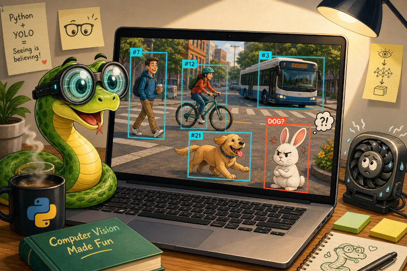
What Is YOLO?

YOLO stands for “You Only Look Once”. The name describes the original idea: process an image with one neural-network pass rather than a slower sequence of separate detection stages.

An object detector answers two questions:

1. What objects are visible?

2. Where is each object?

Its result usually contains a class such as person, a confidence score, and four coordinates that define a bounding box. Other YOLO tasks return different structures. A segmentation model traces the pixels belonging to an object. A pose model finds body keypoints. A classification model assigns a label to the complete image.

Ultralytics puts these tasks behind one Python interface. At the time of writing, the official examples use YOLO26. Older Ultralytics checkpoints, including YOLO11 and YOLOv8 models, remain common in existing projects. Check the package page on PyPI before pinning a version because the project releases often.

Installing Only What We Need

The package installs PyTorch and the libraries it needs. A supported NVIDIA GPU can make inference and training much faster, but it is not required for the examples below. A CPU is enough for learning the interface, although the webcam may acquire a slightly philosophical frame rate.

Project 1: Ask a Pre-Trained Model What It Sees

For the first very simple detection:

On the first run, Ultralytics downloads the pre-trained weights. The n in yolo26n.pt means nano, the smallest model in that family. Small models trade some accuracy for lower memory use and faster inference, which makes them a sensible starting point.

model(...) returns a list because the input may contain more than one image. Each item is a Results object. Calling show() opens the annotated image.

The command-line version looks like this:

yolo predict model=yolo26n.pt source="https://ultralytics.com/images/bus.jpg"

The command saves its output under runs/detect/predict by default. The Ultralytics CLI uses argument=value, not the more usual --argument value form.

One Source Argument, Several Kinds of Input

The source parameter accepts paths, URLs, directories, NumPy arrays, PIL images, videos, webcam indices, and lists of images:

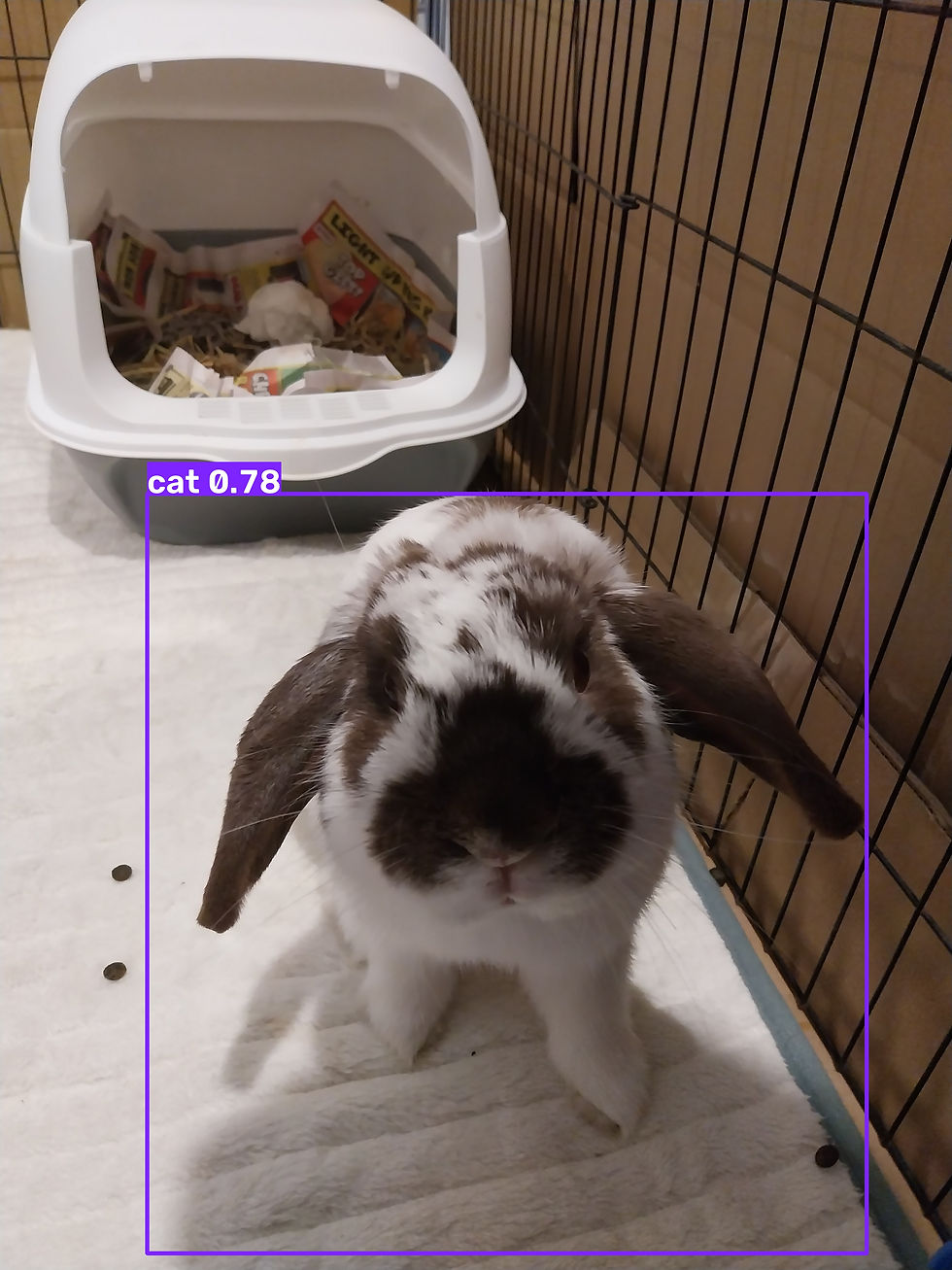
Since we did not explicitly train this model, it mill most likely detect the bunny as a dog or cat in this case.

For a long video or live feed, use stream=True. Ultralytics then returns a generator rather than retaining every result in memory:

A two-hour recording may contain hundreds of thousands of frames. Streaming lets us process one result at a time without teaching the computer a painful lesson about exhausted memory.

Turning the Result Back into Data

Coloured rectangles are satisfying, but most applications need the values behind them. Detection results expose coordinates, classes, and confidence scores through result.boxes:

The four values in xyxy are the top-left and bottom-right pixel coordinates. If we need normalised centre coordinates, box.xywhn provides them.

The complete result can also move into friendlier formats:

The result API supports CSV output, crops, NumPy conversion, and movement between CPU and GPU. The prediction documentation lists the fields for each task.

Project 2: Count Selected Objects

Suppose a fixed camera watches a bunny pen. A basic count needs only a class filter:

This counts detections in one frame. It does not know whether a bunny in frame 20 is the same bunny in frame 21. It would happily count one bunny several thousand times and feel no embarrassment about the result. For video, we need tracking.

Project 3: Give Video Objects Persistent IDs

Tracking assigns an ID to each object and tries to keep that ID across frames. Ultralytics supports tracking with detection, segmentation, and pose models:

The parameter persist=True tells the tracker that the next frame belongs to the same sequence. Track IDs support line-crossing counters, dwell-time estimates, sports analysis, and visitor counts. Ultralytics documents BoT-SORT and ByteTrack on its tracking page.

The word persistent needs some restraint. An ID is a tracker hypothesis, not a biometric identity. Occlusion, missed detections, a camera cut, or two similar objects crossing can cause an ID switch. An object that leaves and returns may receive a new number.

This means len(set(track_ids)) is not automatically a reliable count of people. It is a count of track identities produced under one model, tracker, threshold, and video. That distinction matters as soon as somebody makes decisions based on these numbers.

Detection Is Only One Task

Changing the checkpoint changes the result we receive.

Instance Segmentation

Segmentation gives each detected object a pixel mask. It suits background removal, visible-area measurement, and separating overlapping items:

The resulting image will look something along these lines

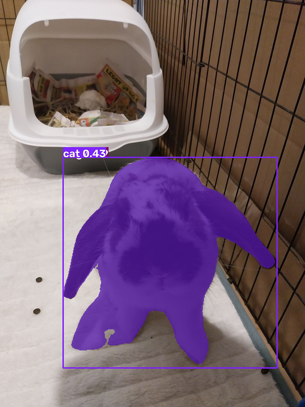
Image Classification

Classification labels the whole image rather than locating each object. A product-photo sorter may need only this task:

In this case the model thinks that with a probability of close to 14%, my bunny is an Old English Sheepdog, followed by nearly 10% with the probability to be a Siberian Husky.

Pose Estimation

A pose model finds keypoints such as shoulders, elbows, hips, and knees. Those points can support exercise-form feedback, gesture experiments, or sports analysis:

Oriented Bounding Boxes

Normal boxes stay horizontal. Oriented bounding-box models rotate the box to fit the object, which helps with aerial imagery, ships, documents, and long objects placed at an angle:

The Ultralytics task overview compares detection, segmentation, classification, pose, semantic segmentation, depth, and oriented boxes.

The Confidence Threshold Is a Decision, Not a Fact

Real inputs are messy, so prediction behaviour needs adjustment:

A higher conf threshold removes weak detections but may hide difficult objects. A larger imgsz can help with small objects, although it costs time and memory. Neither setting turns into a generally correct number because it appeared in one successful notebook.

Suppose a shelf image contains twelve products. At conf=0.25, the model finds eleven and invents two in the background. At conf=0.60, it finds eight and invents none. A human review queue may tolerate extra candidates. An automatic stock alert may not.

The model only supplies scores, but the application turns those scores into decisions.

Project 4: Build a Small Photo Audit

This folder audit records which photos contain a cat or dog, saves annotated previews, and writes a JSON report:

In this case it checks how often my bunny is detected as a cat and how often as a dog. Turns out for the model he looks more like a cat, I always thought he is more like a dog.

The model performs the vision work, while ordinary Python applies the business rule. It also exposes what the detector does not know. The report does not prove that every bunny in the images was found. It does not distinguish a real dog from a mislabeled bunny unless the training data supports that distinction.

Where the Pre-Trained Model Can Go Wrong

A standard checkpoint knows the classes in its training dataset. It may know car, but not a bunny, or the difference between a company vehicle and a visitor’s car. It may know bottle, but not whether the bottle has the correct cap.

Published sample images also tend to be well lit and composed. A fixed camera may produce glare, motion blur, compression artefacts, extreme angles, or tiny distant objects. We need images from the intended environment.

Confidence is a model score, not a direct probability that a claim is true. Calibration can vary by class and input. A detection with 0.87 should not become an 87 per cent real-world guarantee.

Finally, inference is only one part of application latency. Video decoding, resizing, data transfer, drawing, storage, and network calls take time too. The complete application needs benchmarking on the intended hardware.

Final Thoughts

The first project sent several input types through one pre-trained detector. The second treated bounding boxes as ordinary Python data. The third added identities across frames. The fourth combined model output with an application rule.

The progression was:

image → annotated picture

into:

image or video → structured result → application decision

Pre-trained models can recognise only the classes they learned during training. If our object is a cracked tile, a specific circuit-board component, or the neighbour’s escaped cockatoo, the stock model probably needs help.

Part II builds that custom detector, validates it, and exports it for use outside a Python notebook.