pyhctsa: From Feature Matrix to Useful Model, Part II

Part I introduced pyhctsa’s unusually broad approach to time-series measurement. We extracted hundreds of candidate descriptions from each signal and ended with a pandas DataFrame.

That table is the start of the analysis. Some operations fail on particular signals. Feature scales can differ by orders of magnitude. Many columns measure related behaviour, and an enthusiastic classifier can overfit all of them.

This part builds a complete workflow on synthetic data where we know the underlying dynamics. We will use noisy oscillations, autocorrelated signals, and white noise. The goal is to see whether pyhctsa can turn those differences into an interpretable feature space.

I don't really understand why ChatGPT thinks this image summarises the post, but oh well...

Build a dataset with different dynamics

Each sample will contain 1,000 observations. We vary the parameters within each class so the classifier cannot memorise a single waveform.

The raw series already look different, which is useful as a sanity check:

White noise should have little serial dependence. The AR(1) process should retain short-term memory, while the oscillation should produce clear spectral and periodic structure. Looking something like this

Those are exactly the kinds of differences represented across pyhctsa’s correlation, spectral, model-fit, entropy, and nonlinear operations.

Start focused, then widen the search

The full pyhctsa configuration is useful for broad discovery, but calculating thousands of features can take time. During development, it is often better to start with a focused configuration that tests a few plausible views of the signals.

Our synthetic classes differ mainly in serial dependence, predictability, periodicity, and irregularity. Correlation and entropy operations therefore provide a sensible first pass.

Create a file named exploration.yaml:

correlation:
  first_crossing:
    base_name: first_crossing
    ordered_args: [corr_fun, threshold, what_out]
    configs:
      - corr_fun: ac
        threshold: [0, "1/e"]
        what_out: both
        zscore: true

entropy:
  sample_entropy:
    base_name: sample_entropy
    ordered_args: [m, r]
    configs:
      - m: 2
        r: [0.1, 0.2]
        zscore: true
        select: sampen2

      - m: 3
        r: [0.1, 0.2]
        zscore: true
        select: sampen3

Load it through the same calculator interface:

The autocorrelation crossings estimate how quickly dependence decays. The sample-entropy measurements describe the regularity or unpredictability of each signal at several parameter settings. These features should respond differently to white noise, a persistent AR(1) process, and a noisy oscillation.

This focused run is not intended to find every useful distinction. It is a quick way to verify the dataset, labels, extraction process, and downstream analysis before paying the computational cost of the full library.

If the small set does not reveal enough structure, widen the search using pyhctsa’s packaged configuration:

The broad configuration lets correlation, entropy, spectral, nonlinear, model-based, symbolic, and other operation families compete as descriptions of the data. It is particularly useful when you do not yet know which kind of dynamics separates the classes.

A practical workflow moves in both directions:

1. Begin with a focused configuration while building and checking the pipeline.

2. Run the broad configuration to discover informative measurements.

3. Inspect the operations behind the strongest features.

4. Save those operations and parameter choices in a smaller YAML file.

5. Use that reduced configuration for repeated experiments or production extraction.

The custom file is more than a performance optimisation. It records which measurements produced the feature matrix, making the analysis easier to reproduce and audit.

Clean the feature matrix

Feature extraction across diverse methods produces a few awkward outputs. A calculation may return infinity, fail for a short or unsuitable signal, or produce the same value in every row.

For modelling, keep finite numeric columns that vary:

Dropping a column after one missing value is conservative. On a larger and less controlled dataset, you may prefer an imputer. Fit that imputer inside each cross-validation fold, like a scaler, to prevent information from the held-out data entering the training process.

Do not delete failed rows without checking them. If most features fail on one recording, the raw signal may contain NaN, infinity, too few samples, or no variation. That is a data-quality finding rather than an inconvenience to hide.

Scale features without letting outliers take over

Time-series features do not share a natural unit. One column may contain probabilities between zero and one, another a time lag, and another an error with a long-tailed distribution.

Scikit-learn’s RobustScaler centres each feature on its median and scales it using the interquartile range. Extreme feature values have less influence than they would under mean and standard-deviation scaling.

For a visualisation based on the whole dataset, fitting once is fine. Predictive evaluation requires stricter handling. The scaler must learn from the training fold only. We will enforce that with a scikit-learn pipeline later.

Look at the feature space

PCA gives us a quick view of the dominant directions in the feature matrix.

PCA does not know the class labels. Separation means the feature measurements capture differences that dominate the dataset’s overall variance. In this case the result would look similar to the following

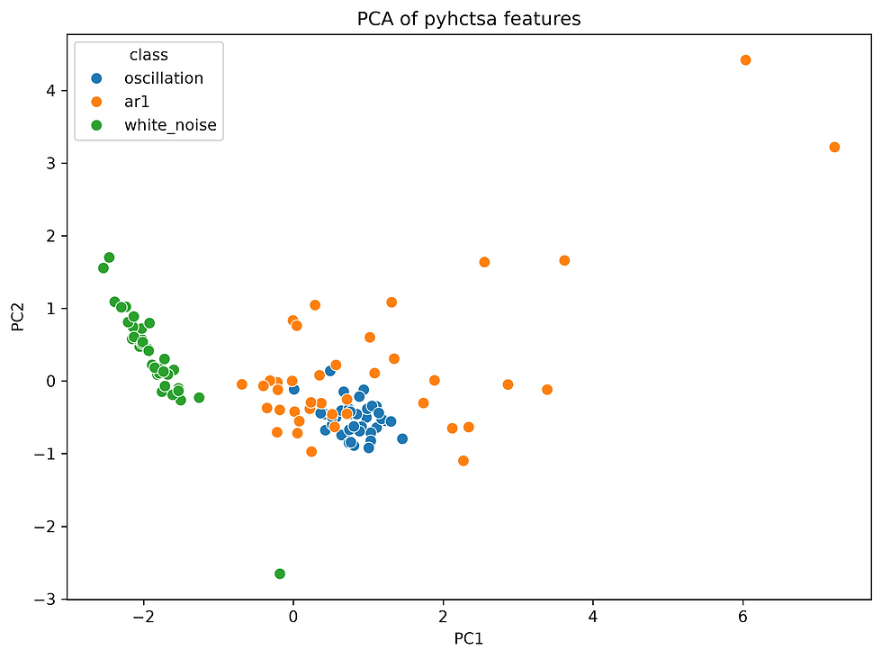
Overlap does not prove the features are useless; a supervised model may use a direction that PCA discards.

You can add t-SNE for a second view:

t-SNE is an exploratory plot, not evidence of classifier performance. In this case it will look like this

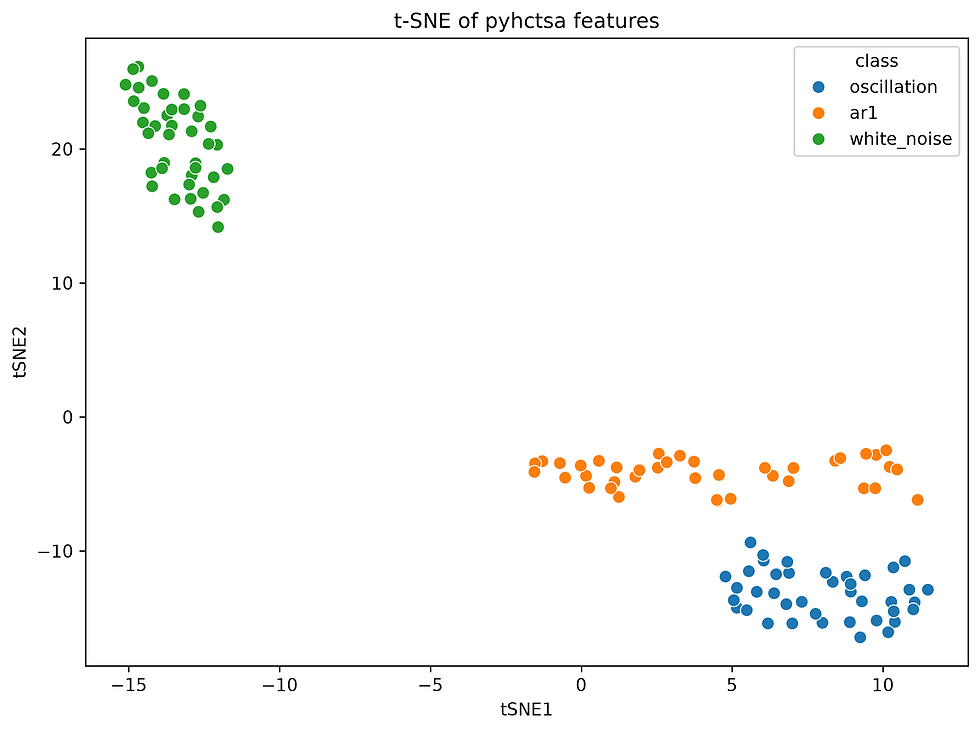
Its neighbourhoods depend on settings and random initialisation. Keep the fixed seed and compare it with PCA and cross-validation.

Classification without data leakage

We will use a linear support vector classifier. A linear model is a good match for this exercise because we can inspect which features receive large coefficients.

The scaler fits inside a pipeline with the classifier:

The pipeline refits RobustScaler inside each training fold. The test fold remains unseen until scoring. This distinction is easy to miss because scaling has no class labels, but its medians and spreads still contain information about held-out samples.

Our synthetic samples are independent. With recordings from people, machines, or experiments, ordinary random folds can leak identity. If several windows came from the same subject, use GroupKFold or StratifiedGroupKFold and keep each subject in one fold.

from sklearn.model_selection import StratifiedGroupKFold

group_cv = StratifiedGroupKFold(
    n_splits=5,
    shuffle=True,
    random_state=42,
)

# groups contains one subject or machine ID per row.
# scores = cross_validate(
#     model, X, target, groups=groups, cv=group_cv
# )

Find the features the model uses

Fit the pipeline on the complete dataset after cross-validation has given you an honest performance estimate. Then inspect the linear coefficients.

This will test all the features, either from the small 8 example configuration or the whole suite of features, and perform a LinearSVC. The final table tells you the highest coefficient, or really its absolute value, for any of the features and how they appear. In case of the whole lot of features this might look as follows

walker_prop_0p5.res_runstest                  0.005938
tc3_mi.raw                                    0.005517
transition_matrix_quantile_3_1.maxeig         0.005388
tc3_mi.denom                                  0.004637
sample_entropy_5_0p1.meanchsampen             0.004079
tc3_2.abs                                     0.003990
surprise_dist_5_tau_embed2quadrants_500.lq    0.003977
transition_matrix_quantile_5_ac.maxeig        0.003963
embed_pca_mi_10.perc_2                        0.003891
tc3_mi.abs                                    0.003862
automutual_info_stats_40_gaussian.ami32       0.003775
walker_prop_1p1.res_runstest                  0.003748 

In case of looking through all possible features, you end up with close to 5000, so this would be quite meaningless.

Roughly said, you can see how important they are for at least one of the time series. In other words, large coefficients identify the columns that influence at least one class decision. Correlated features can share or exchange weight, so the list is not a unique explanation.

A box plot connects a selected measurement back to the classes:

Now the long feature name becomes useful. It often points to the operation family and parameter choices. Import the corresponding function, read its docstring, and inspect the underlying signals. The model has narrowed a large library to a short research list.

For a more stable ranking, repeat the fitting across validation folds and count how often a feature appears near the top. You can also use permutation importance on held-out folds, although correlated columns will still complicate interpretation.

Parallel extraction for larger collections

The full feature set can be expensive. pyhctsa includes a local process distributor built on pathos:

Set the worker count near the number of physical CPU cores, then measure memory use. Each worker needs access to the feature functions and a chunk of signals. More workers can make a memory-constrained machine slower.

Parallelism helps when you have enough series to distribute. For one or two short signals, process startup may cost more time than it saves.

Note that if this option is taken, you need to use the freeze_support() function from multiprocessing package.

Cache the expensive step

Feature extraction is deterministic for most configured operations, so save the raw result before cleaning it. Parquet works well when all columns are numeric. A pickle preserves mixed error strings if you need to audit failures.

Store the configuration beside the results and record the package version. This becomes important when a configuration changes or the package adds an operation. A saved DataFrame without its version and YAML file is hard to reproduce.

What this workflow can become

Classification is one use. The same matrix supports several kinds of analysis:

• Cluster unlabelled recordings and inspect which features distinguish the groups.

• Fit an anomaly detector to known healthy signals, then rank unusual recordings.

• Regress a continuous target such as temperature, fatigue, or remaining component life.

• Track selected features over rolling windows to find changes in dynamics.

• Compare feature distributions before and after an intervention.

The interpretation step stays the same. Use the broad library to find responsive measurements, check those measurements against the raw series, and rerun the analysis with a smaller configuration.

pyhctsa puts many traditions of time-series analysis behind one extraction interface. The result fits familiar pandas and scikit-learn workflows, but the columns retain links to autocorrelation, entropy, spectral structure, symbolic dynamics, model fits, and other concrete ideas about how signals behave.

The package helps you turn an open-ended question about dynamics into a short list of measurements you can plot, test, and explain.