Optimisation with Pyomo, Part I: What Should We Make When Resources Run Out?

Most data work ends with a chart. Then someone asks: “So what should we do?”

That question is where optimisation begins.

This is a two-part series about mathematical optimisation in Python, using Pyomo. It is neither a maths course nor a solver benchmark. The goal is to learn how to formulate a decision problem, read the answer critically, and know when the answer should not be trusted.

In this first part we build the smallest useful model, solve it, and learn to read what the solver tells us. In Part II we make the model more realistic, and watch the answer change in ways that are slightly uncomfortable.

Apparently chairs have 5 legs for ChatGPT...perhaps it should not be asked to run the design department yet.

The Workshop

We go for a very simple setup first. A small workshop makes two products: chairs and tables.

Each week it has a fixed amount of wood, machine time and finishing time. Each product uses some of each, and earns some profit.

	Chair	Table	Available per week
Profit	30	70
Wood (m²)	2	5	40
Machine (hours)	1	2	18
Finishing (hours)	3	2	36

The question: how many chairs and tables should we make each week?

Tables earn more per unit, but they eat wood. Chairs are cheap on wood, but they need a lot of finishing. Intuition gets you as far as “some mix of both”. Finding the best mix is the actual job.

Three Ingredients

Every optimisation model has the same three parts.

1. Decision variables. The things we are free to choose. Here: the number of chairs c and tables t.

2. An objective. The single number we want to make as large (or small) as possible. Here: total profit.

3. Constraints. The rules every acceptable choice must obey. Here: wood, machine and finishing limits.

Written as maths, the workshop looks like this:

maximise    30c + 70t

subject to  2c + 5t ≤ 40     (wood)
            1c + 2t ≤ 18     (machine)
            3c + 2t ≤ 36     (finishing)
            c, t ≥ 0

Every expression is a straight line. That makes this a linear programme. The word “programming” in linear programming here means planning, and is older than Python by several decades. It comes from the original concept of optimising a logistical plan or schedule.

The hard part of optimisation is deciding which variables, objective and constraints describe the problem. Solving it comes after that. The software optimises exactly what we write down, and nothing else.

The Model Is Not the Solver

Pyomo is a modelling library. It lets us describe the problem in Python. It does not solve anything itself.

A solver, a separate program, does the number-crunching. Pyomo hands the model over and reads the answer back.

For this series we use HiGHS, an open-source solver. Older tutorials often use GLPK or CBC. Both work, but they are separate programs that you install through your operating system. The nice thing about the split is that the model code does not care. Switching solvers later means changing one string.

This separation is probably the most useful design decision in the whole library.

The Smallest Useful Model

Here is the workshop, translated line by line:

ConcreteModel means the model is built immediately, from values we already have. That is the simplest option, and the right one for this series.

NonNegativeReals says each variable may be any number from zero upwards, including fractions. That is an obvious problem in our question, we will have to deal with later.

The expressions look like ordinary Python, but they are not evaluated. For example model.chairs is a symbolic variable, so 30 \* model.chairs + 70 \* model.tables builds an expression tree that the solver can inspect.

We gave it an objective in the form of our expression and that it should maximize this. Then we added contstraints, written in the same way as we wood when formulating the problem in the first place.

We gave every constraint a name so we can use it to ask questions about the answer.

Solving It

To solve the problem we simply add

This will give us the answer

optimal
chairs: 9.09
tables: 4.36
profit: 578.18

The solver says the best weekly plan is about 9.09 chairs and 4.36 tables, for a profit of 578.18.

Yes, 9.09 chairs is obviously a problem and we will have to come back to that in Part II. There is a difference between optimising for any solution and optimising for integer solutions.

First, notice the line that printed optimal. That is the solver telling us it proved the answer cannot be beaten. We will see in a moment that this word is not guaranteed.

Reading the Answer: Binding and Slack

The profit number alone does not explain why the plan looks like this. For that, we need to read the constraints.

Which results in

wood       used 40.00 of 40   slack 0.00
machine    used 17.82 of 18   slack 0.18
finishing  used 36.00 of 36   slack 0.00

Wood and finishing time are used up completely. We call those constraints binding. They are the bottlenecks that decide the plan.

Machine time has a little slack left over. Nothing is limiting us there, so adding more machine hours would not change the answer at all.

Reading the constraints tells us something the profit number alone could not: wood and finishing limit the workshop. Buying a faster machine would be money wasted. This is a common outcome. In a linear optimisation problem without any integrality constraint, an optimal solution, if it exists, will be on a corner of the polygon described by the constraining inequalities. This is of course does not mean that it is satisfies every constraint as an equality, but it will satisfy some of them.

The Picture

With only two variables, we can draw the whole problem.

Each constraint becomes a line, and each line gives a ceiling on tables for a given number of chairs. The shaded polygon underneath all three ceilings is the feasible region: every plan that obeys every rule.

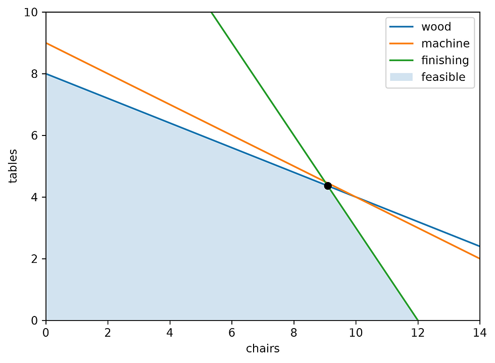
The black dot is our solution. It sits on a corner, exactly where the wood and finishing lines cross. The machine line passes just above it, which is the 0.18 of slack from earlier.

For a linear problem, the best answer always sits at a corner of the feasible region. Solvers exploit that: they hop from corner to corner, always uphill, until no neighbouring corner is better.

Two variables make a flat picture. Two thousand variables make a polytope nobody can visualise, but the idea is the same. This is also the reason why such problems can be solved in the first place.

Shadow Prices

Managers will want to know: “What would one more unit of wood be worth?”

The solver can tell us. Before solving, we declare a Suffix that imports the dual values:

This results in

wood        13.64
machine      0.00
finishing    0.91

These are shadow prices. One extra square metre of wood is worth about 13.64 in profit. One extra finishing hour is worth about 0.91. Extra machine time is worth nothing, which matches the slack we saw earlier.

The model can help with buying decisions too. If a supplier offers wood at 10 per square metre, the model says yes. At 15, it says no.

One caution: shadow prices are marginal. They hold for small changes. Add enough wood and a different constraint becomes the bottleneck, and the price changes. You can see that well in the image, adding sufficient amount of wood, will make the machine constraint relevant and essentially replace the wood constraint.

We will see exactly that happen in Part II.

The solver’s receipt

There is a lovely check hiding in these numbers. Multiply each binding limit, our previous amount for the optimal solution, by its shadow price and add them up:

The result is exactly the optimal profit.

Combining the wood and finishing constraints with these weights produces 30c + 70t ≤ 578.18 for every feasible plan. The shadow prices are the proof that nothing better exists. We can check the solver’s receipt instead of taking its word for it.

When Things Go Wrong

So far the solver has always said optimal. In real work it often will not, and two failures are worth knowing by name.

Infeasible means the constraints contradict each other, so no plan satisfies all of them. Unbounded means the objective can improve forever, which almost always means a constraint is missing.

By default, Pyomo tries to load a solution into the model even when there is not a good one. A safer pattern is to check the status first:

Let us break the workshop on purpose. A customer demands 13 chairs, but finishing time only allows 12:

And a model with no ceiling on what we can make:

The habit worth building: never read variable values before checking the termination condition. A solver that stopped early still hands you numbers, but they are not an answer.

When NOT to Use This

Optimisation can be more machinery than a problem needs.

If there is one product and one scarce resource, the answer is a division. If you have a handful of options, a loop is enough. A spreadsheet with a few rows may be easier to explain to the person who has to approve the plan.

Optimisation earns its place when the choices interact: when more of one thing means less of another, across several limits at once. Once intuition struggles to keep up with those interactions, a solver starts paying for its setup cost.

It also fails quietly when the model is wrong. The solver will happily find the best answer to a question you did not mean to ask.

Where We Are

We now have a working model, and we can interpret it. We know which resources limit the workshop, what an extra unit of each is worth, and how to detect a solver that did not actually finish.

We also have a result that no carpenter would accept: 9.09 chairs and 4.36 tables.

In Part II we deal with that by forcing the model to think in whole units. We will restructure the model so data flows in from tables, add a customer commitment, sweep the wood supply, and discuss what the model still does not know.

Since we are dedicating a Part II to it, simply rounding the solution will obviously not give the best integral solution in all cases.