Mixle: Ask the Fitted Model More Than One Question — Part II

In Part I, we used Mixle to fit two kinds of latent structure. The first was a two-component Gaussian mixture for request latency, while the second was a Dirichlet-process mixture whose observations contained continuous values, categories, counts, collections, and sequences.

Both examples ended with groups, which makes it look a bit like Mixle is a flexible clustering library. This is a bit of a wrong impression, so we want to fix it here.

A fitted probability model can score an observation, generate synthetic observations, expose latent probabilities, and become a component inside a larger model. Those operations support anomaly detection, topic discovery, hidden-state analysis, predictive checking, and several kinds of uncertainty-aware workflow.

The questions for this part are:

What can we do with a fitted density besides draw its curve?

and

When does a shared probabilistic interface become more useful than a collection of specialised estimators?

We will build two more small projects: heterogeneous anomaly detection for API events and topic discovery in a synthetic document collection. We will then use model sampling as a diagnostic, sketch sequence and regression extensions, and decide when Mixle is solving a real problem rather than merely providing an impressive number of import paths.

No idea, why ChatGPT thought this image would summarize the post ...

Density Turns “Unusual” into a Model-Relative Quantity

Anomaly detection is often introduced as a search for extreme values. That works when unusual means “far from the centre of one numeric column”. It becomes less useful when a row is unusual only because several individually ordinary values occur together.

Consider three API-event fields:

duration_ms | endpoint | retries

A duration of 180 milliseconds is ordinary for checkout and slow for search.

Three retries may be unusual for every endpoint, but especially suspicious when combined with a very slow response.

The anomaly therefore belongs to the joint record, not to one universal threshold on one column. A fitted joint density gives us a model-relative score:

high log density → familiar under the fitted model
low log density  → unusual under the fitted model

The phrase “under the fitted model” is essential.

Low density does not mean malicious, broken, fraudulent, or important. It means the observation is surprising to a particular model trained on a particular reference dataset.

At best we can call this useful evidence, but it is not proof for anything.

Project 3: Find Unusual API Events as Complete Records

We will create normal API events with four endpoints:

The ordinary event generator makes latency depend on endpoint:

This just randomly selects and endpoint, generates a fitting duration with a log normalizes normal distribution and then a number of retries with a poisson distribution, although the parameter changes if we are looking at the "checkout" endpoint.

We train on 900 ordinary events. The test set contains another 270 ordinary events and 30 deliberately injected anomalies with much larger latency and retry counts:

This is not a realistic incident simulator. It is a controlled test of whether a model trained on heterogeneous normal behaviour assigns low density to records that violate that behaviour.

Letting Mixle Propose the Joint Model

The entire training call is short:

For the seeded dataset, Mixle 0.7.0 returned:

HeterogeneousBayesianNetwork(
    fields=3,
    edges=[1->0]
)

Field 1 is the endpoint and field 0 is duration. The selected edge represents the dependence we built into the data: latency changes by endpoint.

It should not be read as a causal discovery result. The generator used endpoint to choose a latency distribution, but an automatically fitted edge in real observational data would still need domain reasoning before anyone gave it a causal interpretation.

A density model needs the joint distribution. It does not automatically explain the system that created it.

Scoring Each Record

The model exposes log_density(...) directly:

We define an anomaly threshold from the lower one per cent of the training-score distribution:

This is an empirical decision rule. It simply says that a new event is flagged when its log density is lower than 99 per cent of the reference events used for training.

The choice of one per cent is not delivered by any theory. In our case this is a pure gut feeling decision. A real threshold should reflect investigation capacity, event frequency, costs of false positives and false negatives, temporal drift, and the degree to which the training period genuinely represents normal operation.

Measuring the Demonstration Rather Than Admiring It

Because we injected the anomalies ourselves, we can calculate precision and recall:

The seeded run produced:

Training-score 1% cutoff: -11.793
Flagged: 33
True positives: 30
False positives: 3
Precision: 0.909
Recall: 1.000

All 30 injected anomalies were found, together with three ordinary events. That strong result is unsurprising because the injected events were deliberately dramatic. Their latency and retry patterns sit far outside the training distribution.

A more useful next test would introduce difficult anomalies:

• a search request with checkout-like latency but no retries;

• a normal latency paired with an unusual endpoint-retry combination;

• a gradual latency drift rather than one isolated extreme;

• a novel endpoint that the categorical model has never seen;

• bursts of correlated events that are individually plausible.

An anomaly detector becomes interesting where the cases stop volunteering.

Inspecting the Least Likely Events

Scores become more useful when returned beside the original fields:

The ten least likely events in this run were all injected anomalies. The lowest-scoring row combined a checkout duration above 1.1 seconds with multiple retries.

The ranking matters more than the decimal form of the score.

Raw log density depends on the model family, field structure, units, and observation dimensionality. It should usually be interpreted relative to a comparable reference distribution rather than treated as a universal severity scale.

Drawing the Score Distribution

The figure sorts test events by log density and marks the injected anomalies separately:

Mixle anomaly scores for heterogeneous API events

The anomalies form a very low-density group on the left.

The ordinary test events mostly remain above the cutoff, although three cross it. Those false positives are not necessarily modelling errors. A one-per-cent training threshold is designed to flag a small tail of normal-looking reference behaviour as well.

The operational question is whether the ranking helps an investigator spend attention better than a collection of separate column thresholds.

Sampling Is a Diagnostic, Not Merely a Party Trick

The high-level fitted model can generate new records:

That lets us compare model-generated data with the training data.

This is a simple predictive check. If the model has learned the joint structure, synthetic rows should reproduce important patterns without copying the original rows one by one.

We can compare endpoint counts, median latency, and mean retries (training table is just our training set from above as a dataframe):

For the seeded run, selected values were:

Training data
endpoint   n    median_ms   mean_retries
cart       149  137.5       0.060
checkout    60  179.4       0.217
product    260   95.7       0.108
search     431   74.0       0.081

Synthetic data
endpoint   n    median_ms   mean_retries
cart       179  140.3       0.084
checkout    68  187.1       0.074
product    285   99.6       0.060
search     468   75.8       0.079

The latency medians and endpoint frequencies are reasonably reproduced. It is not perfect, but at least it comes close. On the other hand, the checkout retry rate is not reproduced at all. The fitted Bayesian network included an endpoint-to-duration edge but no endpoint-to-retries edge. Its synthetic checkout events therefore lose much of the elevated retry behaviour built into the generator.

This is exactly why sampling matters. The anomaly scores looked excellent on the deliberately easy test. The synthetic check found a structural weakness that precision and recall on those anomalies did not reveal.

A fitted model can pass one test and still fail another. Generating from it lets the failure speak in the same units as the original data.

Project 4: Discover Topics as Probability Distributions over Words

A topic model treats each document as a mixture of latent topics and each topic as a probability distribution over words. This is another latent-variable problem, but the observations no longer look like customer rows or API events. Instead we have sparse word counts.

The Mixle repository includes latent models such as LDA, and the notebook collection contains broader text and language examples. We will use a deliberately small synthetic corpus so that the recovered themes can be checked without downloading an external dataset.

Creating Three Overlapping Themes

The vocabulary contains programming, football (world cup is just going on), and cooking terms (I like to eat):

VOCABULARY = [
    "python", "data", "model", "pandas", "chart",
    "goal", "team", "match", "coach", "league",
    "recipe", "oven", "flavour", "bread", "kitchen",
]

Each theme has five core words with different probabilities:

THEMES = [
    (
        ["python", "data", "model", "pandas", "chart"],
        [0.24, 0.24, 0.20, 0.18, 0.14],
    ),
    (
        ["goal", "team", "match", "coach", "league"],
        [0.25, 0.24, 0.22, 0.15, 0.14],
    ),
    (
        ["recipe", "oven", "flavour", "bread", "kitchen"],
        [0.24, 0.22, 0.20, 0.18, 0.16],
    ),
]

For each document, 85 per cent of tokens come from its main theme and 15 per cent are noise from the full vocabulary.

Mixle’s LDA example represents a document as sorted (word, count) pairs:

This sparse representation avoids repeating every token in the object passed to the estimator. To generate the documents we use the following.

The complete generator creates 80 documents per theme. Fills them with either the words from the theme 85% of the time or some other words from our very short vocabulary. Then we already add the sorted word/count pairs.

Fitting the LDA Model

We request three categorical topic distributions:

Unlike the Dirichlet-process mixture in Part I, this model receives the number of topics explicitly.

That choice belongs to the analysis. Three is appropriate because the corpus was generated from three themes. On real text, topic count should be investigated through held-out performance, stability, coherence, domain usefulness, and sensitivity analysis rather than selected because a three-panel figure fits nicely on a screen.

Reading the Top Words

Each fitted topic is a categorical distribution with a probability map:

The seeded fit recovered:

Topic 1: goal, team, match, coach, league
Topic 2: recipe, oven, flavour, bread, kitchen
Topic 3: python, data, model, pandas, chart

The order of topics is arbitrary. Mixle did not learn that football is ontologically Topic 1, even though it should since the world cup is going on at the moment of writing this. It learned three categorical word distributions, and our labels were added afterwards by reading their highest-probability words.

This is the same label-switching issue encountered with ordinary mixtures.

Latent components receive meaning from their fitted distributions and the surrounding domain, not from their integer index.

Plotting the Topic Distributions

The figure uses the five highest-probability words from each topic:

Three topics recovered by Mixle LDA

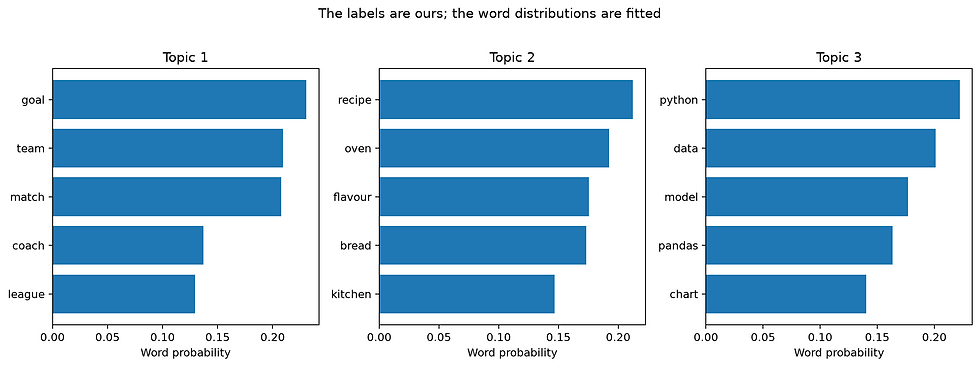
The separation is clean because the corpus was designed to be kind.

Real documents will be far less cooperative. Words are polysemous, topics overlap, document lengths vary, named entities dominate, and bag-of-words representations ignore order and syntax.

A topic distribution can summarise recurring vocabulary, but it should not be mistaken for a complete representation of meaning.

The Same Interface Extends to Sequences

The probabilistic-programming layer can express a two-state Gaussian hidden Markov model with one line of model structure:

This changes the latent structure. A mixture assumes that observations receive component labels without a temporal transition process. An HMM adds state persistence and transition probabilities, so neighbouring observations influence the hidden-state interpretation.

That is appropriate for machine modes, behavioural states, weather regimes, language segments, and similar sequence problems.

It is unnecessary when observations are exchangeable rows. A hidden Markov model should not be added because the data happened to be stored in time order. It should be added because state transitions are part of the process we are trying to represent.

The PPL Surface Also Covers Priors and Regression

A parameter position in mixle.ppl can contain a fixed value, free, another distribution used as a prior, or an expression involving data fields.

A prior on a Gaussian mean can be written as:

Here the standard deviation is fixed at 1.0. The mean on the other hand is in itself an unknown quantity, but with some information. Namely it is normally distributed around 0 with a standard deviation of 10.

A regression mean can be constructed from named fields:

These examples reveal why Mixle’s compositional idea matters. The mean of a distribution is not restricted to one stored number. It can be estimated, assigned a prior, or made into an expression over observed fields.

Of course this way of constructing the multiple linear regression will only be useful if having it as a probabilistic model is useful later on. Otherwise you can just simply use a regression from your favourite library.

The inference route then follows the resulting structure. The model can report that route with explain_fit() rather than requiring the reader to guess whether a fit used closed-form updates, expectation-maximisation, variational inference, or a sampling method.

That is an attractive design and creates a larger surface area to learn than a library dedicated to one model family.

Moving the Calculation Is Not the Same as Improving the Model

Mixle separates model structure from compute engines and distributed backends.

The official examples include patterns such as:

and:

This is useful when the same likelihood and sufficient-statistic calculations genuinely need a different device or execution system. We definitely should not use Spark for our 900 API events.

The architecture notebooks make the same broader point: encode once, reuse work, choose an engine that matches the data size, and reach for sharding when the data rather than the novelty requires it.

For example, a GPU can accelerate a bad assumption and a cluster can distribute it across several machines, but they will not repair or magically fix the model.

Mixle Beside More Familiar Tools

No single comparison captures every model in the package, but the following distinctions are useful.

Need	Often simpler choice	Where Mixle becomes interesting
Fit one standard distribution	SciPy	The distribution must compose with records, mixtures, priors, or sequences
Numeric Gaussian mixture	scikit-learn	Components contain heterogeneous or nested distributions
Standard supervised prediction	scikit-learn, XGBoost, PyTorch	A joint density, sampling, latent structure, or uncertainty-aware composition is central
General Bayesian modelling	PyMC, NumPyro, Stan	Mixle’s built-in distribution catalogue and shared fit/engine abstractions match the intended structure
Topic modelling	Gensim, scikit-learn	LDA needs to sit beside other Mixle latent or heterogeneous models in one workflow
Large distributed tabular processing	Spark or Dask directly	The same fitted probabilistic structure must move between local and distributed execution

This is not a winner’s table. PyMC and Stan have mature Bayesian workflows and diagnostics. Scikit-learn has an enormous supervised-learning ecosystem and familiar interfaces. SciPy is difficult to improve upon when the task is simply to evaluate or fit one known family.

Mixle’s strongest argument is compositional consistency. That argument matters only when the problem needs the composition. So for many ordinary applications Mixle is probably quite a bit out there as the default solution. Many times a more "standard" library might be the better fit.

Important Limitations

The package is marked Beta

Mixle 0.7.0 is classified as Beta on PyPI. The project is moving quickly, and interfaces or defaults may change. So it would be wise to pin versions for reproducible work and preserve fitted artefacts together with package metadata.

Windows is listed as untested

The PyPI installation notes describe Linux as CI-tested and macOS as the day-to-day development platform, while Windows is untested. That does not prove it will fail on Windows, but it changes how confidently the environment can be recommended.

Automatic model selection can automate the wrong abstraction

A selected distribution family or dependency graph is still a modelling choice. Inspect it, challenge it, and compare it against domain-informed alternatives.

Log density is sensitive to representation

Changing units, field encodings, sequence lengths, or included variables changes the score. An anomaly threshold belongs to one model and one input contract.

Mixtures and latent models can be unstable

Local optima, label switching, redundant components, and weak identifiability do not disappear because the fitting call is short.

Generated data can reproduce unwanted structure

A sampler reflects the model, including biases and errors learned from the training set. Synthetic does not mean safe, anonymous, representative, or fair.

More inference routes create more diagnostic obligations

EM, MAP, variational inference, MCMC, and NUTS do not provide interchangeable forms of certainty. The result must be interpreted according to the route that produced it.

Final Thoughts

The anomaly project used one fitted model to score complete API events. The sampling check used that same model to reveal a dependency it had not preserved. The topic project changed the observation type entirely, but still fitted latent probability distributions and inspected their components.

This is the main reason Mixle is interesting.

The package does not merely collect many statistical models under one namespace. It tries to make them behave like compatible pieces:

fit → score → sample → inspect → compose

That consistency can reduce glue code and make unusual model combinations practical.

It can also conceal a large amount of statistical machinery behind a small call. The correct response is neither automatic trust nor automatic suspicion. But rather to keep asking the fitted model different questions. A useful model should not only recognise the data it has seen.

It should survive being asked to explain, generate, compare, and occasionally contradict itself.